An ANOVA report with table of descriptives, diagnostic tests and ANOVA-specific statistics.
Analysis of Variance or ANOVA is a statistical procedure that tests equality of means for several samples. It was first introduced in 1921 by famous English statistician Sir Ronald Aylmer Fisher.
One-Way ANOVA was carried out, with Gender as independent variable, and Internet usage in leisure time (hours per day) as a response variable. Factor interaction was taken into account.
In order to get more insight on the model data, a table of frequencies for ANOVA factors is displayed, as well as a table of descriptives.
Below lies a frequency table for factors in ANOVA model. Note that the missing values are removed from the summary.
| gender | N | % | Cumul. N | Cumul. % |
|---|---|---|---|---|
| male | 410 | 60.92 | 410 | 60.92 |
| female | 263 | 39.08 | 673 | 100 |
| Total | 673 | 100 | 673 | 100 |
The following table displays the descriptive statistics of ANOVA model. Factor levels lie on the left-hand side, while the corresponding statistics for response variable are given on the right-hand side.
| Gender | Min | Max | Mean | Std.Dev. | Median | IQR |
|---|---|---|---|---|---|---|
| male | 0 | 12 | 3.27 | 1.953 | 3 | 3 |
| female | 0 | 12 | 3.064 | 2.355 | 2 | 3 |
| Skewness | Kurtosis |
|---|---|
| 0.9443 | 0.9858 |
| 1.398 | 1.87 |
Before we carry out ANOVA, we'd like to check some basic assumptions. For those purposes, normality and homoscedascity tests are carried out alongside several graphs that may help you with your decision on model's main assumptions.
| Method | Statistic | p-value |
|---|---|---|
| Lilliefors (Kolmogorov-Smirnov) normality test | 0.168 | 3e-52 |
| Anderson-Darling normality test | 18.75 | 7.261e-44 |
| Shapiro-Wilk normality test | 0.9001 | 1.618e-20 |
So, the conclusions we can draw with the help of test statistics:
based on Lilliefors test, distribution of Internet usage in leisure time (hours per day) is not normal
Anderson-Darling test confirms violation of normality assumption
according to Shapiro-Wilk test, the distribution of Internet usage in leisure time (hours per day) is not normal
As you can see, the applied tests confirm departures from normality of the Internet usage in leisure time (hours per day).
In order to test homoscedascity, Bartlett and Fligner-Kileen tests are applied.
| Method | Statistic | p-value |
|---|---|---|
| Fligner-Killeen test of homogeneity of variances | 0.4629 | 0.4963 |
| Bartlett test of homogeneity of variances | 10.77 | 0.001032 |
When it comes to equality of variances, applied tests yield inconsistent results. While Fligner-Kileen test confirmed the hypotheses of homoscedascity, Bartlett's test rejected it.
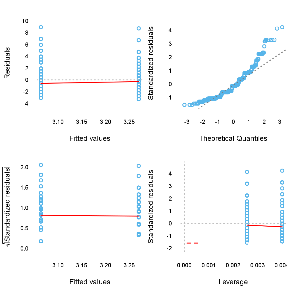
Here you can see several diagnostic plots for ANOVA model:
| Df | Sum.Sq | Mean.Sq | F.value | Pr..F. | |
|---|---|---|---|---|---|
| gender | 1 | 6.422 | 6.422 | 1.43 | 0.2322 |
| Residuals | 636 | 2856 | 4.49 |
F-test for Gender is not statistically significant, which implies that there is no Gender effect on response variable.
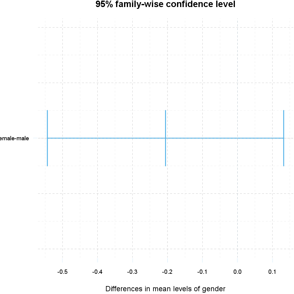
After getting the results of the ANOVA, usually it is advisable to run a post hoc test to explore patterns that were not specified a priori. Now we are presenting Tukey's HSD test.
| Difference | Lower Bound | Upper Bound | |
|---|---|---|---|
| female-male | -0.206 | -0.543 | 0.132 |
| P value | |
|---|---|
| female-male | 0.232 |
There are no categories which differ significantly here.
Below you can see the result of the post hoc test on a plot.
An ANOVA report with table of descriptives, diagnostic tests and ANOVA-specific statistics.
Analysis of Variance or ANOVA is a statistical procedure that tests equality of means for several samples. It was first introduced in 1921 by famous English statistician Sir Ronald Aylmer Fisher.
Two-Way ANOVA was carried out, with Gender and Relationship status as independent variables, and Internet usage in leisure time (hours per day) as a response variable. Factor interaction was taken into account.
In order to get more insight on the model data, a table of frequencies for ANOVA factors is displayed, as well as a table of descriptives.
Below lies a frequency table for factors in ANOVA model. Note that the missing values are removed from the summary.
| gender | partner | N | % | Cumul. N | Cumul. % |
|---|---|---|---|---|---|
| male | in a relationship | 150 | 23.7 | 150 | 23.7 |
| female | in a relationship | 120 | 18.96 | 270 | 42.65 |
| male | married | 33 | 5.213 | 303 | 47.87 |
| female | married | 29 | 4.581 | 332 | 52.45 |
| male | single | 204 | 32.23 | 536 | 84.68 |
| female | single | 97 | 15.32 | 633 | 100 |
| Total | Total | 633 | 100 | 633 | 100 |
The following table displays the descriptive statistics of ANOVA model. Factor levels and their combinations lie on the left-hand side, while the corresponding statistics for response variable are given on the right-hand side.
| Gender | Relationship status | Min | Max | Mean | Std.Dev. |
|---|---|---|---|---|---|
| male | in a relationship | 0.5 | 12 | 3.058 | 1.969 |
| male | married | 0 | 8 | 2.985 | 2.029 |
| male | single | 0 | 10 | 3.503 | 1.936 |
| female | in a relationship | 0.5 | 10 | 3.044 | 2.216 |
| female | married | 0 | 10 | 2.481 | 1.967 |
| female | single | 0 | 12 | 3.323 | 2.679 |
| Median | IQR | Skewness | Kurtosis |
|---|---|---|---|
| 2.5 | 2 | 1.324 | 2.649 |
| 3 | 2 | 0.862 | 0.1509 |
| 3 | 3 | 0.7574 | 0.08749 |
| 3 | 3 | 1.383 | 1.831 |
| 2 | 1.75 | 2.063 | 5.586 |
| 3 | 3.5 | 1.185 | 0.9281 |
Before we carry out ANOVA, we'd like to check some basic assumptions. For those purposes, normality and homoscedascity tests are carried out alongside several graphs that may help you with your decision on model's main assumptions.
| Method | Statistic | p-value |
|---|---|---|
| Lilliefors (Kolmogorov-Smirnov) normality test | 0.168 | 3e-52 |
| Anderson-Darling normality test | 18.75 | 7.261e-44 |
| Shapiro-Wilk normality test | 0.9001 | 1.618e-20 |
So, the conclusions we can draw with the help of test statistics:
based on Lilliefors test, distribution of Internet usage in leisure time (hours per day) is not normal
Anderson-Darling test confirms violation of normality assumption
according to Shapiro-Wilk test, the distribution of Internet usage in leisure time (hours per day) is not normal
As you can see, the applied tests confirm departures from normality of the Internet usage in leisure time (hours per day).
In order to test homoscedascity, Bartlett and Fligner-Kileen tests are applied.
| Method | Statistic | p-value |
|---|---|---|
| Fligner-Killeen test of homogeneity of variances | 1.123 | 0.2892 |
| Bartlett test of homogeneity of variances | 11.13 | 0.0008509 |
When it comes to equality of variances, applied tests yield inconsistent results. While Fligner-Kileen test confirmed the hypotheses of homoscedascity, Bartlett's test rejected it.
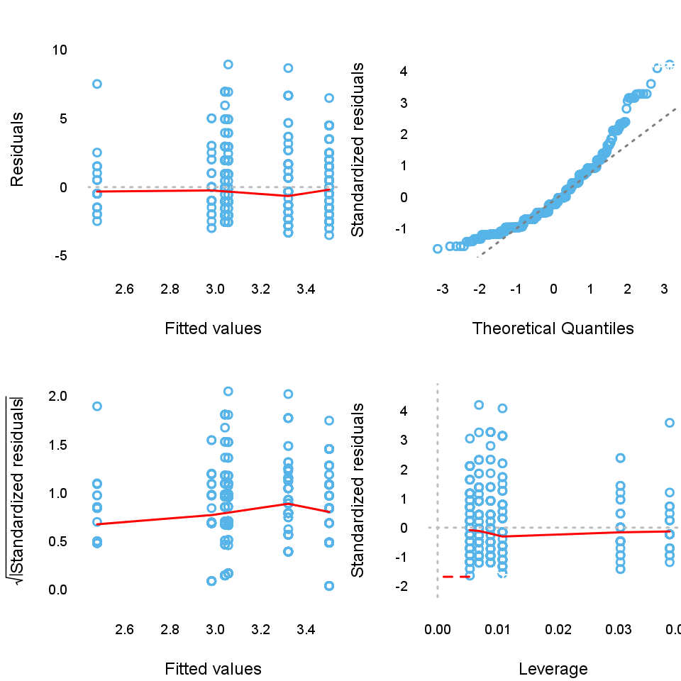
Here you can see several diagnostic plots for ANOVA model:
| Df | Sum.Sq | Mean.Sq | F.value | |
|---|---|---|---|---|
| gender | 1 | 4.947 | 4.947 | 1.085 |
| partner | 2 | 31.21 | 15.61 | 3.424 |
| gender:partner | 2 | 3.038 | 1.519 | 0.3332 |
| Residuals | 593 | 2703 | 4.558 |
| Pr..F. | |
|---|---|
| gender | 0.2979 |
| partner | 0.03324 |
| gender:partner | 0.7168 |
| Residuals |
F-test for Gender is not statistically significant, which implies that there is no Gender effect on response variable. Effect of Relationship status on response variable is significant. Interaction between levels of Gender and Relationship status wasn't found significant (p = 0.717).
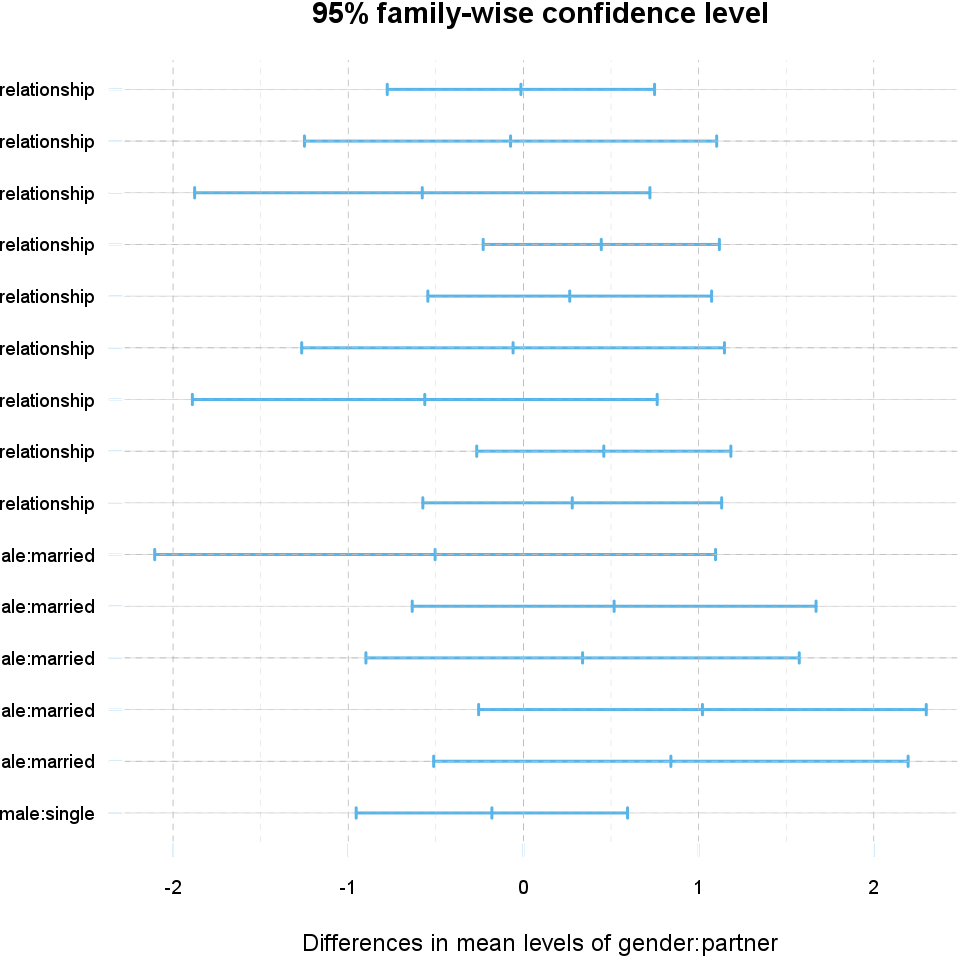
After getting the results of the ANOVA, usually it is advisable to run a post hoc test to explore patterns that were not specified a priori. Now we are presenting Tukey's HSD test.
| Difference | Lower Bound | Upper Bound | |
|---|---|---|---|
| female-male | -0.186 | -0.538 | 0.165 |
| P value | |
|---|---|
| female-male | 0.298 |
There are no categories which differ significantly here.
| Difference | Lower Bound | |
|---|---|---|
| married-in a relationship | -0.289 | -1.012 |
| single-in a relationship | 0.371 | -0.061 |
| single-married | 0.66 | -0.059 |
| Upper Bound | P value | |
|---|---|---|
| married-in a relationship | 0.435 | 0.616 |
| single-in a relationship | 0.803 | 0.109 |
| single-married | 1.379 | 0.079 |
There are no categories which differ significantly here.
| Difference | Lower Bound | |
|---|---|---|
| female:in a relationship-male:in a relationship | -0.014 | -0.777 |
| male:married-male:in a relationship | -0.073 | -1.25 |
| female:married-male:in a relationship | -0.577 | -1.877 |
| male:single-male:in a relationship | 0.444 | -0.23 |
| female:single-male:in a relationship | 0.264 | -0.545 |
| male:married-female:in a relationship | -0.059 | -1.266 |
| female:married-female:in a relationship | -0.563 | -1.89 |
| male:single-female:in a relationship | 0.459 | -0.267 |
| female:single-female:in a relationship | 0.279 | -0.574 |
| female:married-male:married | -0.504 | -2.105 |
| male:single-male:married | 0.518 | -0.635 |
| female:single-male:married | 0.338 | -0.899 |
| male:single-female:married | 1.022 | -0.256 |
| female:single-female:married | 0.842 | -0.512 |
| female:single-male:single | -0.18 | -0.955 |
| Upper Bound | P value | |
|---|---|---|
| female:in a relationship-male:in a relationship | 0.749 | 1 |
| male:married-male:in a relationship | 1.103 | 1 |
| female:married-male:in a relationship | 0.722 | 0.801 |
| male:single-male:in a relationship | 1.119 | 0.412 |
| female:single-male:in a relationship | 1.074 | 0.938 |
| male:married-female:in a relationship | 1.148 | 1 |
| female:married-female:in a relationship | 0.764 | 0.83 |
| male:single-female:in a relationship | 1.184 | 0.461 |
| female:single-female:in a relationship | 1.132 | 0.938 |
| female:married-male:married | 1.097 | 0.946 |
| male:single-male:married | 1.67 | 0.794 |
| female:single-male:married | 1.575 | 0.971 |
| male:single-female:married | 2.3 | 0.201 |
| female:single-female:married | 2.196 | 0.481 |
| female:single-male:single | 0.594 | 0.986 |
There are no categories which differ significantly here.
Below you can see the result of the post hoc test on a plot.
This report was generated with R (3.0.1) and rapport (0.51) in 3.431 sec on x86_64-unknown-linux-gnu platform.