Rapport package team

Description

This template will return the correlation matrix of supplied numerical variables.

Introduction

Correlation is one of the most commonly used statistical tool. With the help of that we can get information about a possible linear relation between two variables. According to the definition of the correlation, one can call it also as the standardized covariance.

The maximum possible value of the correlation (the so-called correlation coefficient) could be 1, the minimum could be -1. In the first case there is a perfect positive (thus in the second case there is a perfect negative) linear relationship between the two variables, though perfect relationships, especially in the social sciences, are quite rare. If two variables are independent from each other, the correlation between them is 0, but 0 correlation coefficient only means certainly a linear independency.

Because extreme values occur seldom we have rule of thumbs for the coefficients, like other fields of statistics:

we call two variables highly correlated if the absolute value of the correlation coefficient between them is higher than 0.7 and
we call them uncorrelated if that is smaller than 0.2.

Please note that correlation has nothing to do with causal models, it only shows association but not effects.

Variable description

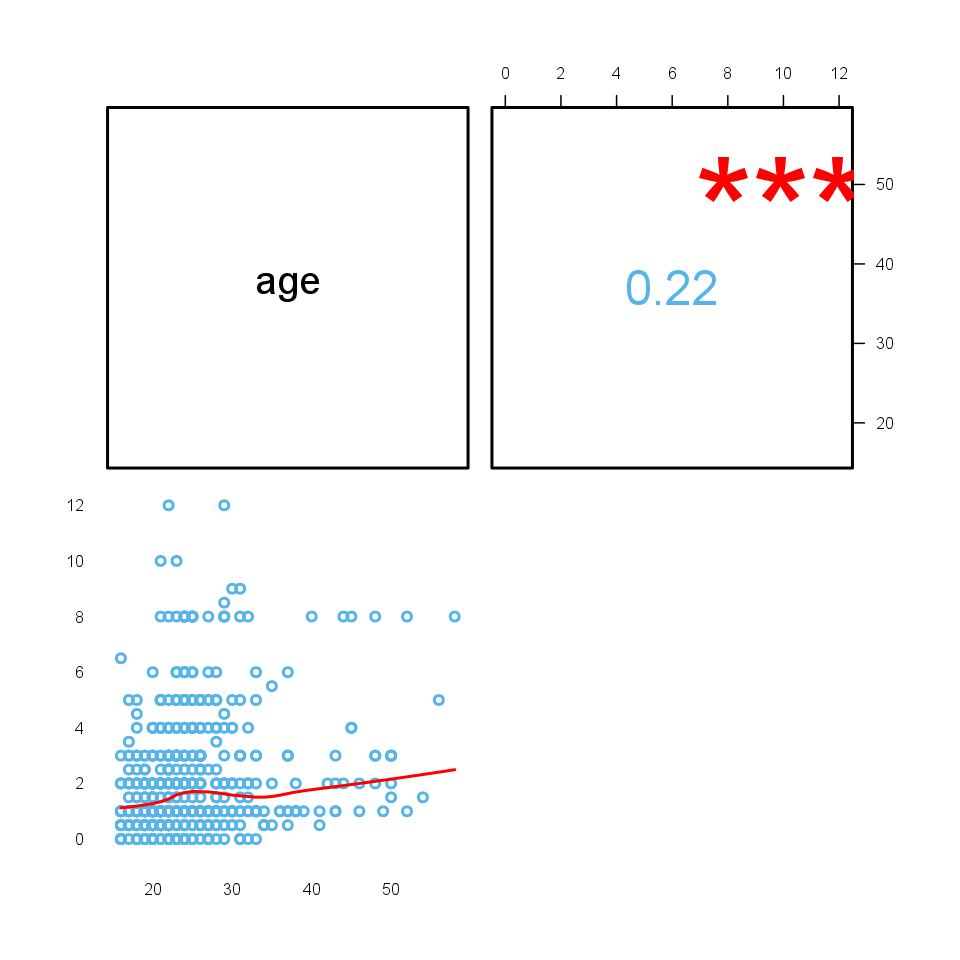
709 variables with 2 cases provided.

There are no highly correlated (r < -0.7 or r > 0.7) variables.

There are no uncorrelated correlated (r < -0.2 or r > 0.2) variables.

Correlation matrix

Correlation matrix
	age	edu
age		0.2185 * * *
edu	0.2185 * * *

Where the stars represent the significance levels of the bivariate correlation coefficients: one star for a p value below 0.05, two for below 0.01 and three for below 0.001.

On the plot one can see the correlation in two forms: below the diagonal visually, above that one can find the coefficient(s).

Description

This template will return the correlation matrix of supplied numerical variables.

Introduction

Because extreme values occur seldom we have rule of thumbs for the coefficients, like other fields of statistics:

we call two variables highly correlated if the absolute value of the correlation coefficient between them is higher than 0.7 and
we call them uncorrelated if that is smaller than 0.2.

Please note that correlation has nothing to do with causal models, it only shows association but not effects.

Variable description

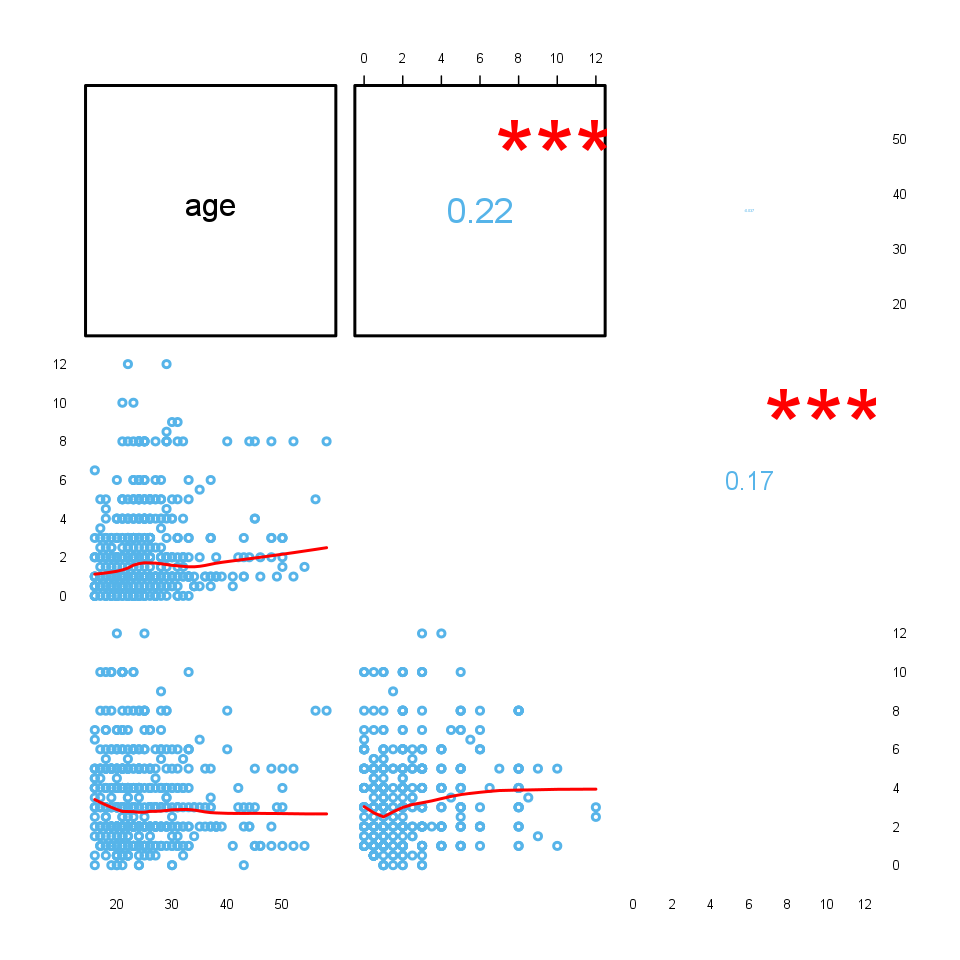
709 variables with 3 cases provided.

The highest correlation coefficient (0.2273) is between edu and age and the lowest (-0.03377) is between leisure and age. It seems that the strongest association (r=0.2273) is between edu and age.

There are no highly correlated (r < -0.7 or r > 0.7) variables.

Uncorrelated (-0.2 < r < 0.2) variables:

leisure and age (-0.03)
leisure and edu (0.17)

Correlation matrix

Correlation matrix
	age	edu	leisure
age		0.2273 * * *	-0.0338
edu	0.2273 * * *		0.1732 * * *
leisure	-0.0338	0.1732 * * *

Where the stars represent the significance levels of the bivariate correlation coefficients: one star for a p value below 0.05, two for below 0.01 and three for below 0.001.

On the plot one can see the correlation in two forms: below the diagonal visually, above that one can find the coefficient(s).

Description

This template will return the correlation matrix of supplied numerical variables.

Introduction

Because extreme values occur seldom we have rule of thumbs for the coefficients, like other fields of statistics:

we call two variables highly correlated if the absolute value of the correlation coefficient between them is higher than 0.7 and
we call them uncorrelated if that is smaller than 0.2.

Please note that correlation has nothing to do with causal models, it only shows association but not effects.

Variable description

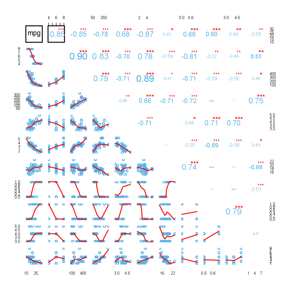
32 variables with 11 cases provided.

The highest correlation coefficient (0.902) is between disp and cyl and the lowest (-0.8677) is between wt and mpg. It seems that the strongest association (r=0.902) is between disp and cyl.

Highly correlated (r < -0.7 or r > 0.7) variables:

cyl and mpg (-0.85)
disp and mpg (-0.85)
hp and mpg (-0.78)
wt and mpg (-0.87)
disp and cyl (0.9)
hp and cyl (0.83)
wt and cyl (0.78)
vs and cyl (-0.81)
hp and disp (0.79)
drat and disp (-0.71)
wt and disp (0.89)
vs and disp (-0.71)
qsec and hp (-0.71)
vs and hp (-0.72)
carb and hp (0.75)
wt and drat (-0.71)
am and drat (0.71)
vs and qsec (0.74)
gear and am (0.79)

Uncorrelated (-0.2 < r < 0.2) variables:

gear and hp (-0.13)
qsec and drat (0.09)
carb and drat (-0.09)
qsec and wt (-0.17)
am and vs (0.17)
carb and am (0.06)

Correlation matrix

Correlation matrix (continued below)
	mpg	cyl	disp
mpg		-0.8522 * * *	-0.8476 * * *
cyl	-0.8522 * * *		0.9020 * * *
disp	-0.8476 * * *	0.9020 * * *
hp	-0.7762 * * *	0.8324 * * *	0.7909 * * *
drat	0.6812 * * *	-0.6999 * * *	-0.7102 * * *
wt	-0.8677 * * *	0.7825 * * *	0.8880 * * *
qsec	0.4187 *	-0.5912 * * *	-0.4337 *
vs	0.6640 * * *	-0.8108 * * *	-0.7104 * * *
am	0.5998 * * *	-0.5226 * *	-0.5912 * * *
gear	0.4803 * *	-0.4927 * *	-0.5556 * * *
carb	-0.5509 * *	0.5270 * *	0.3950 *

Table continues below
	hp	drat	wt
mpg	-0.7762 * * *	0.6812 * * *	-0.8677 * * *
cyl	0.8324 * * *	-0.6999 * * *	0.7825 * * *
disp	0.7909 * * *	-0.7102 * * *	0.8880 * * *
hp		-0.4488 * *	0.6587 * * *
drat	-0.4488 * *		-0.7124 * * *
wt	0.6587 * * *	-0.7124 * * *
qsec	-0.7082 * * *	0.0912	-0.1747
vs	-0.7231 * * *	0.4403 *	-0.5549 * * *
am	-0.2432	0.7127 * * *	-0.6925 * * *
gear	-0.1257	0.6996 * * *	-0.5833 * * *
carb	0.7498 * * *	-0.0908	0.4276 *

Table continues below
	qsec	vs	am
mpg	0.4187 *	0.6640 * * *	0.5998 * * *
cyl	-0.5912 * * *	-0.8108 * * *	-0.5226 * *
disp	-0.4337 *	-0.7104 * * *	-0.5912 * * *
hp	-0.7082 * * *	-0.7231 * * *	-0.2432
drat	0.0912	0.4403 *	0.7127 * * *
wt	-0.1747	-0.5549 * * *	-0.6925 * * *
qsec		0.7445 * * *	-0.2299
vs	0.7445 * * *		0.1683
am	-0.2299	0.1683
gear	-0.2127	0.2060	0.7941 * * *
carb	-0.6562 * * *	-0.5696 * * *	0.0575

	gear	carb
mpg	0.4803 * *	-0.5509 * *
cyl	-0.4927 * *	0.5270 * *
disp	-0.5556 * * *	0.3950 *
hp	-0.1257	0.7498 * * *
drat	0.6996 * * *	-0.0908
wt	-0.5833 * * *	0.4276 *
qsec	-0.2127	-0.6562 * * *
vs	0.2060	-0.5696 * * *
am	0.7941 * * *	0.0575
gear		0.2741
carb	0.2741

Where the stars represent the significance levels of the bivariate correlation coefficients: one star for a p value below 0.05, two for below 0.01 and three for below 0.001.

On the plot one can see the correlation in two forms: below the diagonal visually, above that one can find the coefficient(s).

This report was generated with R (3.0.1) and rapport (0.51) in 4.769 sec on x86_64-unknown-linux-gnu platform.

Rapport package team

Correlations

2011-04-26 20:25 CET

Description

Introduction

Variable description

Correlation matrix

Description

Introduction

Variable description

Correlation matrix

Description

Introduction

Variable description

Correlation matrix