Returning the Chi-squared test of two given variables with count, percentages and Pearson's residuals table.
Two variables specified:
Crosstables are applicable to show the frequencies of categorical variables in a matrix form, with a table view.
We will present four types of these crosstables. The first of them shows the exact numbers of the observations, ergo the number of the observations each of the variables' categories commonly have.
The second also shows the possessions each of these cells have, but not the exact numbers of the observations, rather the percentages of them from the total data.
The last two type of the crosstabs contain the so-called row and column percentages which demonstrate us the distribution of the frequencies if we concentrate only on one variable.
After that we present the tests with which we can investigate the possible relationships, associations between the variables, like Chi-squared test, Fisher Exact Test, Goodman and Kruskal's lambda.
In the last part there are some charts presented, with that one can visually observe the distribution of the frequencies.
| city | small town | village | Missing | Sum | |
|---|---|---|---|---|---|
| male | 338 | 28 | 19 | 25 | 410 |
| female | 234 | 3 | 9 | 17 | 263 |
| Missing | 27 | 2 | 2 | 5 | 36 |
| Sum | 599 | 33 | 30 | 47 | 709 |
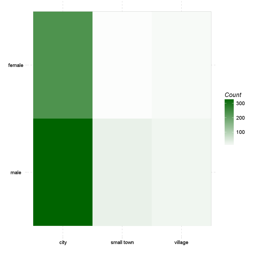
Most of the cases (338) can be found in "male-city" categories. Row-wise "male" holds the highest number of cases (410) while column-wise "city" has the utmost cases (599).
| city | small town | village | Missing | Sum | |
|---|---|---|---|---|---|
| male | 47.67 | 3.95 | 2.68 | 3.53 | 57.83 |
| female | 33 | 0.42 | 1.27 | 2.4 | 37.09 |
| Missing | 3.81 | 0.28 | 0.28 | 0.71 | 5.08 |
| Sum | 84.49 | 4.65 | 4.23 | 6.63 | 100 |
| city | small town | village | Missing | |
|---|---|---|---|---|
| male | 82.44 | 6.83 | 4.63 | 6.1 |
| female | 88.97 | 1.14 | 3.42 | 6.46 |
| Missing | 75 | 5.56 | 5.56 | 13.89 |
| Sum | 84.49 | 4.65 | 4.23 | 6.63 |
| city | small town | village | Missing | Sum | |
|---|---|---|---|---|---|
| male | 56.43 | 84.85 | 63.33 | 53.19 | 57.83 |
| female | 39.07 | 9.09 | 30 | 36.17 | 37.09 |
| Missing | 4.51 | 6.06 | 6.67 | 10.64 | 5.08 |
In the below tests for independece we assume that the row and column variables are independent of each other. If this null hypothesis would be rejected by the tests, then we can say that the assumption must have been wrong, so there is a good chance that the variables are associated.
One of the most widespread independence test is the Chi-squared test. While using that we have the alternative hypothesis, that two variables have an association between each other, in opposite of the null hypothesis that the variables are independent.
We use the cell frequencies from the crosstables to calculate the test statistic for that. The test statistic is based on the difference between this distribution and a theoretical distribution where the variables are independent of each other. The distribution of this test statistic follows a Chi-square distribution.
The test was invented by Karl Pearson in 1900. It should be noted that the Chi-squared test has the disadvantage that it is sensitive to the sample size.
Before analyzing the result of the Chi-squared test, we have to check if our data meets some requirements. There are two widely used criteria which have to take into consideration, both of them are related to the so-called expected counts. These expected counts are calculated from the marginal distributions and show how the crosstabs would look like if there were complete independency between the variables. The Chi-squared test calculates how different are the observed cells from the expected ones.
The two criteria are:
Let's look at on expected values then:
| city | small town | village | |
|---|---|---|---|
| male | 349 | 18.91 | 17.08 |
| female | 223 | 12.09 | 10.92 |
We can see that the Chi-squared test met the requirements.
So now check the result of the test:
| Test statistic | df | P value |
|---|---|---|
| 12.64 | 2 | 0.001804 * * |
To decide if the null or the alternative hypothesis could be accepted we need to calculate the number of degrees of freedom. The degrees of freedom is easy to calculate, we substract one from the number of the categories of both the row and the coloumn variables and multiply them with each other.
To each degrees of freedom there is denoted a critical value. The result of the Chi-square test have to be lower than that value to be able to accept the nullhypothesis.
It seems that a real association can be pointed out between gender and dwell by the Pearson's Chi-squared test (χ=12.64) at the degree of freedom being 2 at the significance level of 0.001804 * *.
The association between the two variables seems to be weak based on Cramer's V (0.1001).
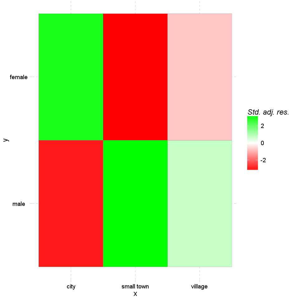
The residuals show the contribution to reject the null hypothesis at a cell level. An extremely high or low value indicates that the given cell had a major effect on the resulting chi-square, so thus helps understanding the association in the crosstable.
| city | small town | village | |
|---|---|---|---|
| male | -3.08 | 3.43 | 0.76 |
| female | 3.08 | -3.43 | -0.76 |
Based on Pearson's residuals the following cells seems interesting (with values higher than 2 or lower than -2):
An other test to check the possible association/independence between two variables, is the Fisher exact test. This test is especially useful with small samples, but could be used with bigger datasets as well.
We have the advantage while using the Fisher's over the Chi-square test, that we could get an exact significance value not just a level of it, thus we can have an impression about the power of the test and the association.
The test was invented by, thus named after R.A. Fisher.
The variables seems to be dependent based on Fisher's exact test at the significance level of 0.0008061 * * *.
With the help of the Goodman and Kruskal's lambda we can look for not only relationship on its own, which have directions if we set one variable as a predictor and the other as a criterion variable.
The computed value for Goodman and Kruskal's lambda is the same for both directions: 0. For this end, we do not know the direction of the relationship.
If one would like to investigate the relationships rather visually than in a crosstable form, there are several possibilities to do that.
At first we can have a look at on the so-called heat map. This kind of chart uses the same amount of cells and a similar form as the crosstable does, but instead of the numbers there are colours to show which cell contains the most counts (or likewise the highest total percentages).
The darker colour is one cell painted, the most counts/the higher total percentage it has.
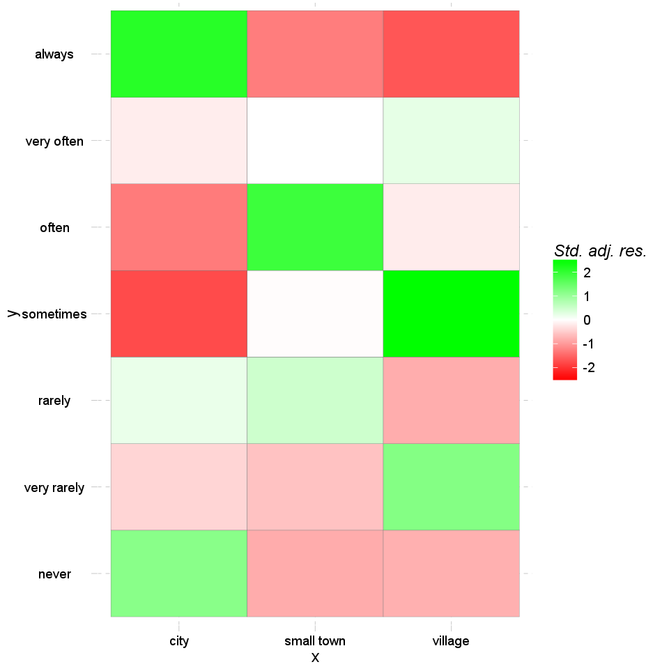
There can be also shown the standardized adjusted residual of each cells:
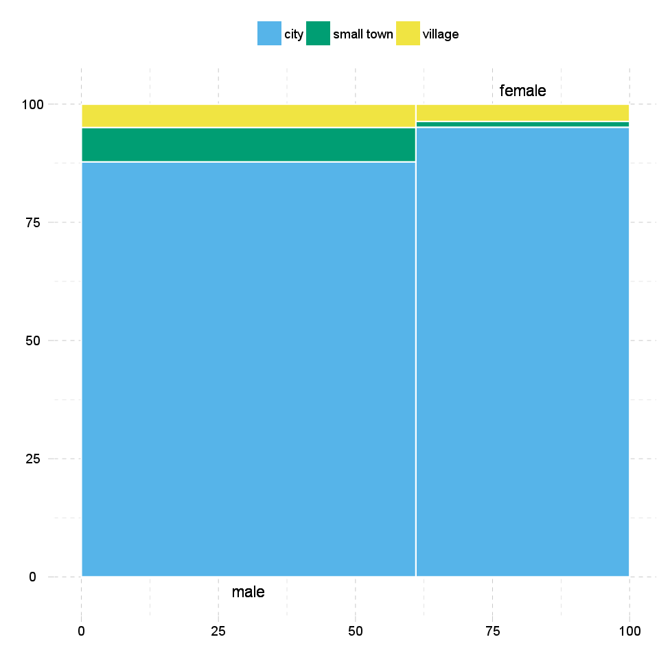
In front of the heat map, on the mosaic charts, not only the colours are important. The size of the cells shows the amount of the counts one cell has.
The width on the axis of gender determinate one side and the height on the axis of the dwell gives the final shape of the box. The box which demonstrates a cell from the hypothetic crosstable. We can see on the top of the chart which category from the dwell draw the boxes what kind of colour.
At last but not least have a glance on the fluctuation diagram. Unlike the above two charts, here the colours does not have influence on the chart, but the sizes of the boxes, which obviously demonstrates here as well the cells of the crosstable.
The bigger are the boxes the higher are the numbers of the counts/the total percentages, which that boxes denote.

Returning the Chi-squared test of two given variables with count, percentages and Pearson's residuals table.
Two variables specified:
Crosstables are applicable to show the frequencies of categorical variables in a matrix form, with a table view.
We will present four types of these crosstables. The first of them shows the exact numbers of the observations, ergo the number of the observations each of the variables' categories commonly have.
The second also shows the possessions each of these cells have, but not the exact numbers of the observations, rather the percentages of them from the total data.
The last two type of the crosstabs contain the so-called row and column percentages which demonstrate us the distribution of the frequencies if we concentrate only on one variable.
After that we present the tests with which we can investigate the possible relationships, associations between the variables, like Chi-squared test, Fisher Exact Test, Goodman and Kruskal's lambda.
In the last part there are some charts presented, with that one can visually observe the distribution of the frequencies.
| city | small town | village | Missing | |
|---|---|---|---|---|
| never | 12 | 0 | 0 | 1 |
| very rarely | 30 | 1 | 3 | 2 |
| rarely | 41 | 3 | 1 | 1 |
| sometimes | 67 | 4 | 8 | 8 |
| often | 101 | 10 | 5 | 7 |
| very often | 88 | 5 | 5 | 10 |
| always | 226 | 9 | 7 | 17 |
| Missing | 34 | 1 | 1 | 1 |
| Sum | 599 | 33 | 30 | 47 |
| Sum | |
|---|---|
| never | 13 |
| very rarely | 36 |
| rarely | 46 |
| sometimes | 87 |
| often | 123 |
| very often | 108 |
| always | 259 |
| Missing | 37 |
| Sum | 709 |
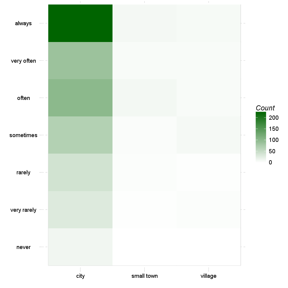
Most of the cases (226) can be found in "always-city" categories. Row-wise "always" holds the highest number of cases (259) while column-wise "city" has the utmost cases (599).
| city | small town | village | Missing | |
|---|---|---|---|---|
| never | 1.69 | 0 | 0 | 0.14 |
| very rarely | 4.23 | 0.14 | 0.42 | 0.28 |
| rarely | 5.78 | 0.42 | 0.14 | 0.14 |
| sometimes | 9.45 | 0.56 | 1.13 | 1.13 |
| often | 14.25 | 1.41 | 0.71 | 0.99 |
| very often | 12.41 | 0.71 | 0.71 | 1.41 |
| always | 31.88 | 1.27 | 0.99 | 2.4 |
| Missing | 4.8 | 0.14 | 0.14 | 0.14 |
| Sum | 84.49 | 4.65 | 4.23 | 6.63 |
| Sum | |
|---|---|
| never | 1.83 |
| very rarely | 5.08 |
| rarely | 6.49 |
| sometimes | 12.27 |
| often | 17.35 |
| very often | 15.23 |
| always | 36.53 |
| Missing | 5.22 |
| Sum | 100 |
| city | small town | village | Missing | |
|---|---|---|---|---|
| never | 92.31 | 0 | 0 | 7.69 |
| very rarely | 83.33 | 2.78 | 8.33 | 5.56 |
| rarely | 89.13 | 6.52 | 2.17 | 2.17 |
| sometimes | 77.01 | 4.6 | 9.2 | 9.2 |
| often | 82.11 | 8.13 | 4.07 | 5.69 |
| very often | 81.48 | 4.63 | 4.63 | 9.26 |
| always | 87.26 | 3.47 | 2.7 | 6.56 |
| Missing | 91.89 | 2.7 | 2.7 | 2.7 |
| Sum | 84.49 | 4.65 | 4.23 | 6.63 |
| city | small town | village | Missing | |
|---|---|---|---|---|
| never | 2 | 0 | 0 | 2.13 |
| very rarely | 5.01 | 3.03 | 10 | 4.26 |
| rarely | 6.84 | 9.09 | 3.33 | 2.13 |
| sometimes | 11.19 | 12.12 | 26.67 | 17.02 |
| often | 16.86 | 30.3 | 16.67 | 14.89 |
| very often | 14.69 | 15.15 | 16.67 | 21.28 |
| always | 37.73 | 27.27 | 23.33 | 36.17 |
| Missing | 5.68 | 3.03 | 3.33 | 2.13 |
| Sum | |
|---|---|
| never | 1.83 |
| very rarely | 5.08 |
| rarely | 6.49 |
| sometimes | 12.27 |
| often | 17.35 |
| very often | 15.23 |
| always | 36.53 |
| Missing | 5.22 |
In the below tests for independece we assume that the row and column variables are independent of each other. If this null hypothesis would be rejected by the tests, then we can say that the assumption must have been wrong, so there is a good chance that the variables are associated.
One of the most widespread independence test is the Chi-squared test. While using that we have the alternative hypothesis, that two variables have an association between each other, in opposite of the null hypothesis that the variables are independent.
We use the cell frequencies from the crosstables to calculate the test statistic for that. The test statistic is based on the difference between this distribution and a theoretical distribution where the variables are independent of each other. The distribution of this test statistic follows a Chi-square distribution.
The test was invented by Karl Pearson in 1900. It should be noted that the Chi-squared test has the disadvantage that it is sensitive to the sample size.
Before analyzing the result of the Chi-squared test, we have to check if our data meets some requirements. There are two widely used criteria which have to take into consideration, both of them are related to the so-called expected counts. These expected counts are calculated from the marginal distributions and show how the crosstabs would look like if there were complete independency between the variables. The Chi-squared test calculates how different are the observed cells from the expected ones.
The two criteria are:
Let's look at on expected values then:
| city | small town | village | |
|---|---|---|---|
| never | 10.83 | 0.6134 | 0.5559 |
| very rarely | 30.69 | 1.738 | 1.575 |
| rarely | 40.62 | 2.3 | 2.085 |
| sometimes | 71.3 | 4.038 | 3.66 |
| often | 104.7 | 5.93 | 5.374 |
| very often | 88.45 | 5.01 | 4.54 |
| always | 218.4 | 12.37 | 11.21 |
We can see that the Chi-squared test met the requirements.
So now check the result of the test:
| Test statistic | df | P value |
|---|---|---|
| 14.86 | 12 | 0.249 |
To decide if the null or the alternative hypothesis could be accepted we need to calculate the number of degrees of freedom. The degrees of freedom is easy to calculate, we substract one from the number of the categories of both the row and the coloumn variables and multiply them with each other.
To each degrees of freedom there is denoted a critical value. The result of the Chi-square test have to be lower than that value to be able to accept the nullhypothesis.
The requirements of the chi-squared test was not met, so Yates's correction for continuity applied. The approximation may be incorrect.
It seems that no real association can be pointed out between email and dwell by the Pearson's Chi-squared test (χ=14.86 at the degree of freedom being 12) at the significance level of 0.249.
The residuals show the contribution to reject the null hypothesis at a cell level. An extremely high or low value indicates that the given cell had a major effect on the resulting chi-square, so thus helps understanding the association in the crosstable.
| city | small town | village | |
|---|---|---|---|
| never | 1.15 | -0.81 | -0.77 |
| very rarely | -0.41 | -0.59 | 1.2 |
| rarely | 0.2 | 0.49 | -0.8 |
| sometimes | -1.75 | -0.02 | 2.49 |
| often | -1.28 | 1.9 | -0.18 |
| very often | -0.17 | 0 | 0.24 |
| always | 2.1 | -1.26 | -1.64 |
Based on Pearson's residuals the following cells seems interesting (with values higher than 2 or lower than -2):
An other test to check the possible association/independence between two variables, is the Fisher exact test. This test is especially useful with small samples, but could be used with bigger datasets as well.
We have the advantage while using the Fisher's over the Chi-square test, that we could get an exact significance value not just a level of it, thus we can have an impression about the power of the test and the association.
The test was invented by, thus named after R.A. Fisher.
The test could not finish within resource limits.
If one would like to investigate the relationships rather visually than in a crosstable form, there are several possibilities to do that.
At first we can have a look at on the so-called heat map. This kind of chart uses the same amount of cells and a similar form as the crosstable does, but instead of the numbers there are colours to show which cell contains the most counts (or likewise the highest total percentages).
The darker colour is one cell painted, the most counts/the higher total percentage it has.
There can be also shown the standardized adjusted residual of each cells:
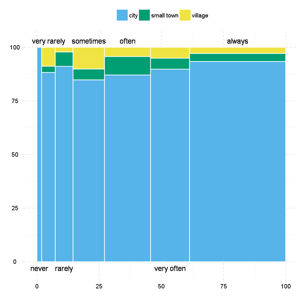
In front of the heat map, on the mosaic charts, not only the colours are important. The size of the cells shows the amount of the counts one cell has.
The width on the axis of email determinate one side and the height on the axis of the dwell gives the final shape of the box. The box which demonstrates a cell from the hypothetic crosstable. We can see on the top of the chart which category from the dwell draw the boxes what kind of colour.
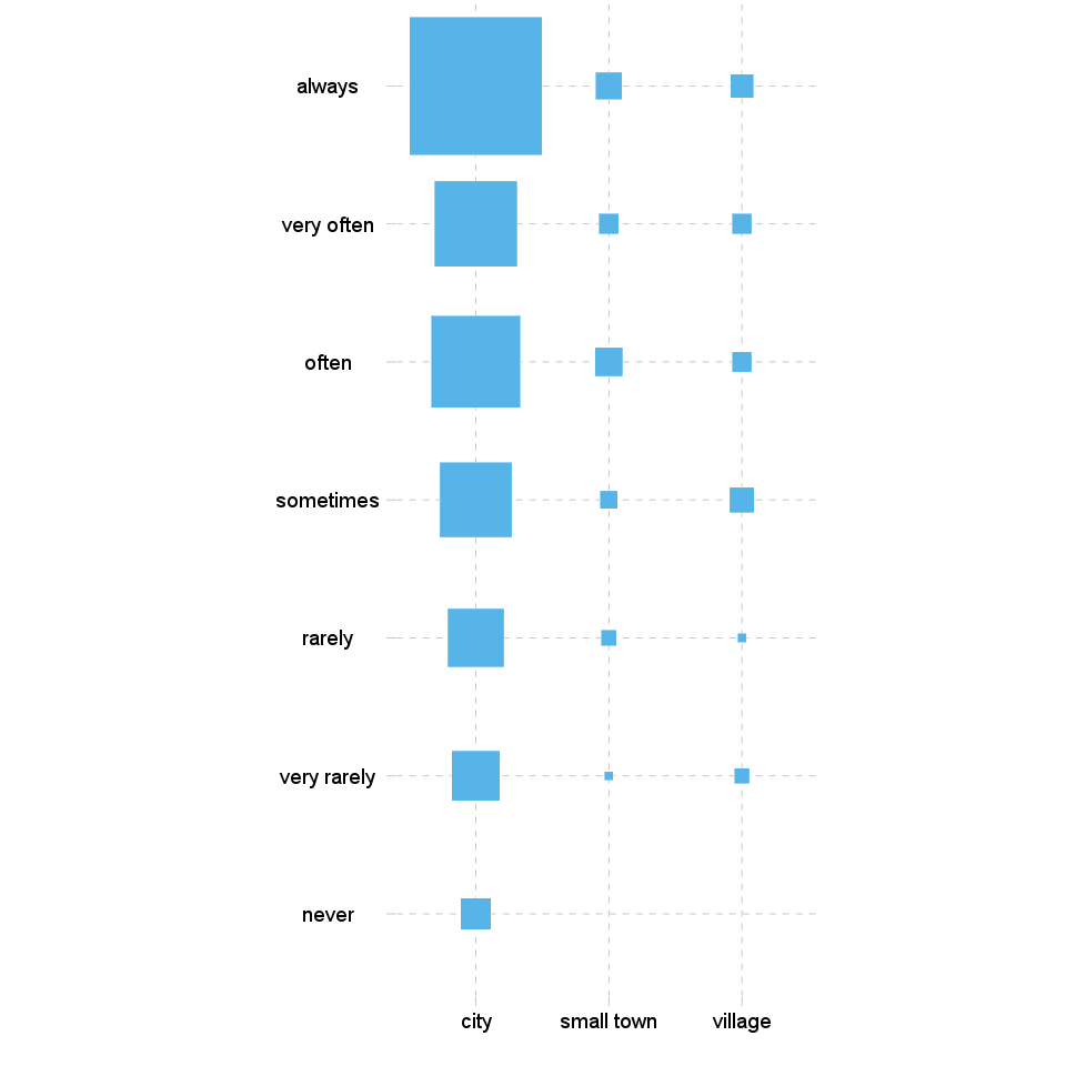
At last but not least have a glance on the fluctuation diagram. Unlike the above two charts, here the colours does not have influence on the chart, but the sizes of the boxes, which obviously demonstrates here as well the cells of the crosstable.
The bigger are the boxes the higher are the numbers of the counts/the total percentages, which that boxes denote.
This report was generated with R (3.0.1) and rapport (0.51) in 7.099 sec on x86_64-unknown-linux-gnu platform.
Logo and design: © 2012 rapport Development Team | License (AGPL3) | Fork on GitHub | Styled with skeleton