K-means clustering with automatically estimated number of clusters
K-means Clustering is a specific and one of the most widespread method of clustering. With clustering we want to divide our data into groups, which in the objects are similar to each other. K-means clustering is specified in the way, here we set the number of groups we want to make. In our case we will take into account the following variables: Age, Internet usage for educational purposes (hours per day) and Internet usage in leisure time (hours per day), to find out which observations are the nearest to each other.
J. B. MacQueen (1967). "Some Methods for classification and Analysis of Multivariate Observations, Proceedings of 5-th Berkeley Symposium on Mathematical Statistics and Probability". 1:281-297
As it was mentioned above, the speciality of the K-means Cluster method is to set the number of groups we want to produce.
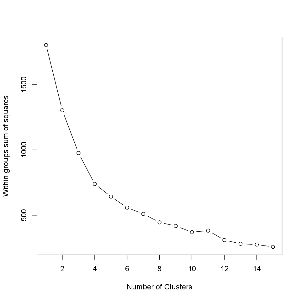
Let's see how to decide which is the ideal number of them!
We can figure out that, as we see how much the Within groups sum of squares decreases if we set a higher number of the groups. So the smaller the difference the smaller the gain we can do with increasing the number of the clusters (thus in this case the larger decreasing means the bigger gain).
The ideal number of clusters seems to be 2.
The method of the K-means clustering starts with the step to set k number of centorids which could be the center of the groups we want to form. After that there comes several iterations, meanwhile the ideal centers are being calculated.
The centroids are the observations which are the nearest in average to all the other observations of their group. But it could be also interesting which are the typical values of the clusters! One way to figure out these typical values is to see the group means. The 2 cluster averages are:
| age | edu | leisure | |
|---|---|---|---|
| 1.Cluster | 0.4092 | 1.285 | 0.9275 |
| 2.Cluster | -0.1251 | -0.393 | -0.2837 |
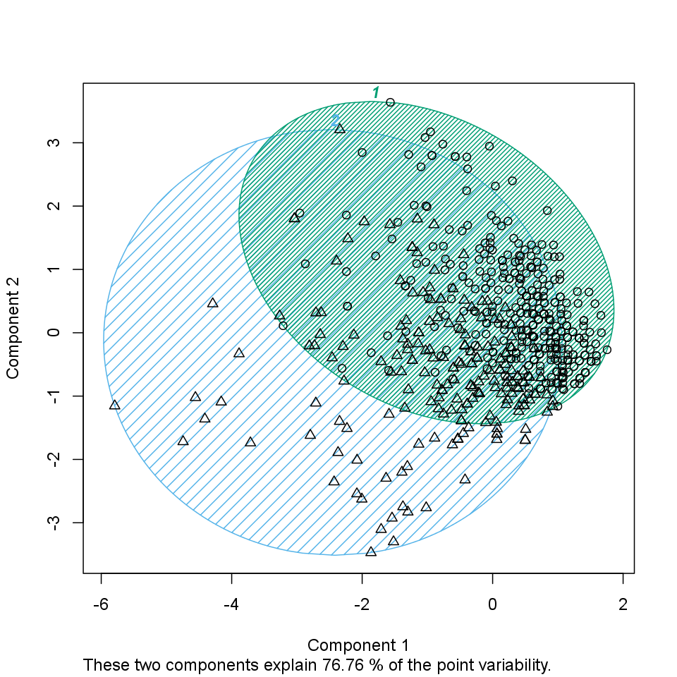
The size of the above clusters are: 141 and 461.
On the chart below we can see the produced groups. To distinct which observation is related to which cluster each of the objects from the same groups have the same figure and there is a circle which shows the border of the clusters.
K-means clustering with automatically estimated number of clusters
K-means Clustering is a specific and one of the most widespread method of clustering. With clustering we want to divide our data into groups, which in the objects are similar to each other. K-means clustering is specified in the way, here we set the number of groups we want to make. In our case we will take into account the following variables: drat, cyl, wt and mpg, to find out which observations are the nearest to each other.
J. B. MacQueen (1967). "Some Methods for classification and Analysis of Multivariate Observations, Proceedings of 5-th Berkeley Symposium on Mathematical Statistics and Probability". 1:281-297
As it was mentioned above, the speciality of the K-means Cluster method is to set the number of groups we want to produce.
Let's see how to decide which is the ideal number of them!

We can figure out that, as we see how much the Within groups sum of squares decreases if we set a higher number of the groups. So the smaller the difference the smaller the gain we can do with increasing the number of the clusters (thus in this case the larger decreasing means the bigger gain).
The ideal number of clusters seems to be 2.
The method of the K-means clustering starts with the step to set k number of centorids which could be the center of the groups we want to form. After that there comes several iterations, meanwhile the ideal centers are being calculated.
The centroids are the observations which are the nearest in average to all the other observations of their group. But it could be also interesting which are the typical values of the clusters! One way to figure out these typical values is to see the group means. The 2 cluster averages are:
| drat | cyl | wt | mpg | |
|---|---|---|---|---|
| 1.Cluster | 0.838 | -1.053 | -0.8794 | 0.946 |
| 2.Cluster | -0.4904 | 0.6649 | 0.3078 | -0.5118 |
| 3.Cluster | -1.016 | 1.015 | 2.169 | -1.37 |
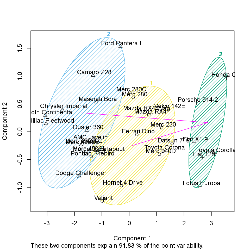
The size of the above clusters are: 13, 16 and 3.
On the chart below we can see the produced groups. To distinct which observation is related to which cluster each of the objects from the same groups have the same figure and there is a circle which shows the border of the clusters.
K-means clustering with automatically estimated number of clusters
K-means Clustering is a specific and one of the most widespread method of clustering. With clustering we want to divide our data into groups, which in the objects are similar to each other. K-means clustering is specified in the way, here we set the number of groups we want to make. In our case we will take into account the following variables: drat, cyl, wt and mpg, to find out which observations are the nearest to each other.
J. B. MacQueen (1967). "Some Methods for classification and Analysis of Multivariate Observations, Proceedings of 5-th Berkeley Symposium on Mathematical Statistics and Probability". 1:281-297
As it was mentioned above, the speciality of the K-means Cluster method is to set the number of groups we want to produce.
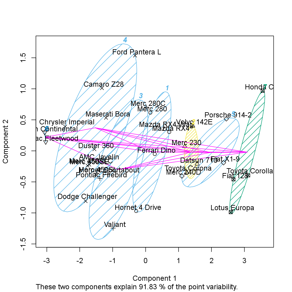
As you set, there will be a 7-means cluster analysis provided.
The method of the K-means clustering starts with the step to set k number of centorids which could be the center of the groups we want to form. After that there comes several iterations, meanwhile the ideal centers are being calculated.
The centroids are the observations which are the nearest in average to all the other observations of their group. But it could be also interesting which are the typical values of the clusters! One way to figure out these typical values is to see the group means. The cluster averages are:
| drat | cyl | wt | mpg | |
|---|---|---|---|---|
| 1.Cluster | -1.265 | -0.105 | 0.1229 | -0.05652 |
| 2.Cluster | -0.8294 | 1.015 | 0.8644 | -0.837 |
| 3.Cluster | 0.3898 | -1.225 | -0.04829 | 0.5823 |
| 4.Cluster | 0.5925 | 0.08166 | -0.1684 | -0.1671 |
| 5.Cluster | 0.8247 | -1.225 | -1.376 | 1.81 |
| 6.Cluster | 2.026 | -1.225 | -1.369 | 1.346 |
| 7.Cluster | 0.5426 | -1.225 | -0.7109 | 0.3002 |
The size of the above clusters are: 2, 13, 2, 6, 4, 2 and 3.
On the chart below we can see the produced groups. To distinct which observation is related to which cluster each of the objects from the same groups have the same figure and there is a circle which shows the border of the clusters.
This report was generated with R (3.0.1) and rapport (0.51) in 8.181 sec on x86_64-unknown-linux-gnu platform.